1. Introduction
Floods are the world's most economically damaging natural hazard and among the deadliest. The CRED EM-DAT database records that floods account for roughly 43% of all reported natural disasters globally, killing an average of 7,000–10,000 people annually over the past three decades. Economic losses routinely exceed $50 billion per year, with significant under-reporting from low- and middle-income countries. In sub-Saharan Africa, floods are the most frequently occurring disaster type, yet the region simultaneously hosts some of the world's least capable flood early warning and monitoring infrastructure.
Quantifying, communicating, and forecasting flood hazard requires a common technical vocabulary — a set of numerical flood indices that translate complex hydrological states into actionable indicators. These indices serve many roles: they define design standards for infrastructure, trigger operational early warnings, calibrate insurance models, and anchor climate change impact assessments. No single index is universally applicable; each reflects a different facet of flood processes — statistical frequency, antecedent wetness, flash potential, inundation extent, or compound hazard.
This article provides a structured review of the principal flood indices in operational and research use, their mathematical derivation, and the global and African forecasting systems that deploy them at temporal scales ranging from nowcasting (0–6 hours) to seasonal outlooks (1–6 months). Particular attention is paid to satellite-based tools that compensate for Africa's declining ground observation network.
This article is intended for hydrology practitioners, water resources engineers, and early warning specialists. Familiarity with basic hydrology — return periods, unit hydrographs, rainfall-runoff modelling — is assumed throughout.
2. A Taxonomy of Flood Indices
2.1 Statistical Streamflow Indices
T-Year Flood Quantile (QT). The most fundamental flood index in water resources engineering. QT is the discharge magnitude with a 1/T annual probability of exceedance — the discharge expected to be exceeded once on average every T years. It is derived by fitting a probability distribution to an Annual Maximum Series (AMS) or Peaks-Over-Threshold (POT) sample, then reading off the T-year quantile. Common distributions include the Generalised Extreme Value (GEV), the Log-Pearson Type III (LP3) — the US standard per Bulletin 17C (England et al., 2019) — and the two-parameter Gumbel (EV1).
σ = scale parameter (σ > 0)
ξ = shape parameter: ξ = 0 → Gumbel; ξ < 0 → bounded upper tail; ξ > 0 → heavy-tailed Fréchet
T = return period (years); note P(Q > QT) = 1/T per year
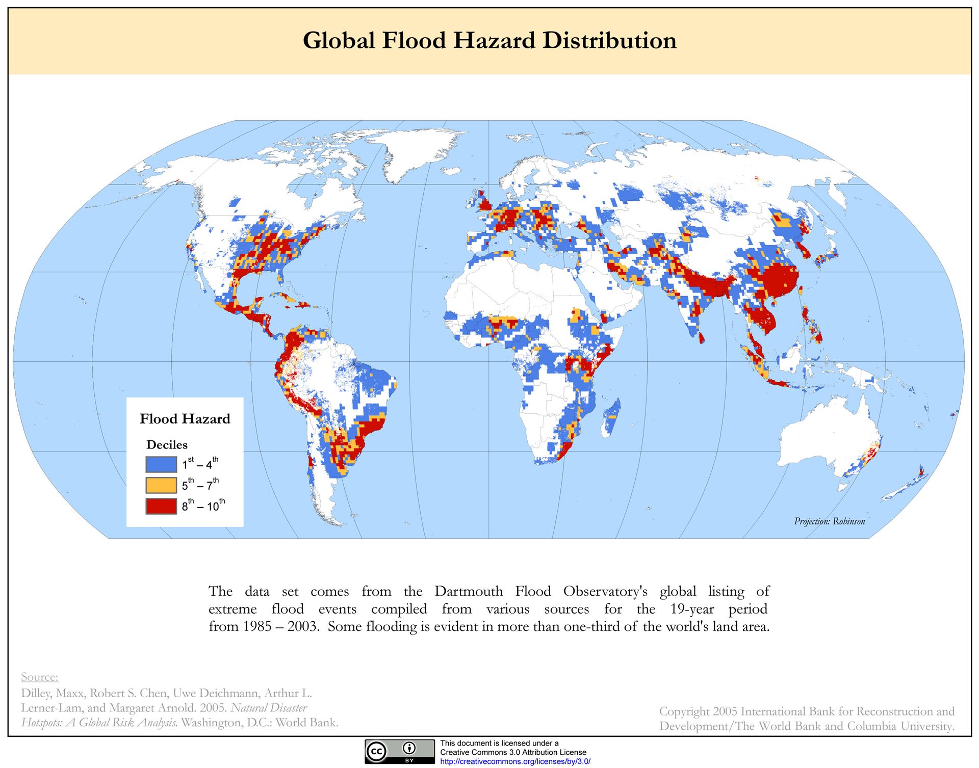
Global Flood Hazard Frequency and Distribution derived from 1985–2003 Dartmouth Flood Observatory extreme flood event data. Warmer colours indicate higher flood frequency — the tropical belt, monsoonal South and Southeast Asia, and sub-Saharan river corridors are clearly the highest-frequency zones globally. This climatological frequency layer underpins the hazard component of FRI and FSI frameworks worldwide. Source: CHRR and CIESIN, Columbia University / NASA SEDAC — CC BY 2.0.
Flood Frequency Ratio (FFR). The dimensionless ratio of an event peak discharge to the long-term mean annual flood Q̄: FFR = Qevent / Q̄. It normalises flows for cross-catchment comparison and underpins the index flood method in regional flood frequency analysis (RFFA) for ungauged basins (Dalrymple, 1960; Hosking & Wallis, 1997).
Bankfull Discharge Ratio. The ratio of event discharge to bankfull channel capacity. Values exceeding 1.0 indicate out-of-bank flooding. Bankfull discharge approximates the 1.5–2.5 year return period flow in natural channels (Leopold et al., 1964) and is a key threshold in real-time flood warning systems.
Base Flow Index (BFI). BFI = Qbase / Qtotal computed over a multi-year period, where Qbase is the baseflow component separated by a digital recursive filter (Lyne & Hollick, 1979; Chapman, 1999). High BFI (>0.7) characterises permeable, slowly responding catchments; low BFI (<0.3) indicates flashy, impermeable terrain with amplified flood peaks. BFI is used in the UK HOST catchment classification (Boorman et al., 1995) and as an input to flood estimation regionalisation methods.
2.2 Rainfall-Derived Indices
Antecedent Precipitation Index (API). First formalised by Kohler & Linsley (1951), API approximates soil moisture state as an exponential decay of prior rainfall:
Pt = precipitation on day t (mm)
Higher API → wetter antecedent conditions → greater proportion of rainfall becoming runoff
Standardized Precipitation Index (SPI). Developed by McKee et al. (1993) and adopted as the WMO standard drought index (Hayes et al., 2011), SPI also serves as a flood precursor at short time scales. A gamma distribution is fitted to precipitation accumulated over a specified window (1, 3, 6, 12, or 24 months), and probabilities are transformed to the standard normal via the equiprobability transformation. SPI ≥ +2.0 denotes extreme wet conditions associated with elevated flood risk.
Standardized Precipitation-Evapotranspiration Index (SPEI). The SPEI (Vicente-Serrano et al., 2010) replaces raw precipitation with the climatic water balance (P − PET), accounting for temperature-driven evaporative demand. It provides a more physically complete indicator of moisture surplus and is increasingly applied in hydro-climatological flood and drought studies, particularly in climate change contexts.
2.3 Flash Flood Indices
Flash Flood Guidance (FFG). Defined as the minimum average rainfall depth of duration τ sufficient to cause bankfull conditions at a point in a basin (Carpenter et al., 1999), FFG integrates current soil moisture state (antecedent deficit) with the unit hydrograph response of the basin. If observed or forecast rainfall P(τ) ≥ FFG(τ), a flash flood threat is declared. The FFG threshold decreases as soils wet up — dynamically coupling antecedent state with warning thresholds in a way that fixed rainfall thresholds cannot.
The WMO Global Flash Flood Guidance System (GFFGS), developed with USAID support, has extended FFG to global coverage through regional implementations covering South Asia, Southeast Asia, the Middle East, Central America, and most critically for this review, sub-Saharan Africa (AfFFGS). These systems use real-time satellite QPE and the Sacramento Soil Moisture Accounting (SAC-SMA) model to update FFG at 6-hourly intervals.
Flash Flood Potential Index (FFPI). A static composite index (scale 1–10) developed by Smith (2003) and operationalised by NOAA/NWS. FFPI weights terrain slope, land cover type, forest canopy density, and soil permeability to map the intrinsic susceptibility of landscapes to rapid runoff generation. Unlike FFG, FFPI does not update dynamically — it characterises climatological potential and is used to spatially prioritise monitoring and warning resources.
2.4 Soil Moisture and Composite Indices
Soil Wetness Index (SWI). Derived from satellite soil moisture observations (ASCAT, SMAP, or SMOS), SWI is the ratio of current soil water content to the observed maximum — ranging from 0 (field dry) to 1 (saturated). Near-surface SWI is propagated downward using an exponential filter (Albergel et al., 2008) to estimate root-zone moisture, which governs the infiltration-runoff partition during events. The Copernicus Global Land Service provides daily SWI maps at 1 km globally.
Standardized Streamflow Index (SSI) / Standardized Runoff Index (SRI). Directly analogous to SPI but applied to observed streamflow or modelled runoff time series (Vicente-Serrano et al., 2012; Shukla & Wood, 2008). SSI > +2.0 signals extreme high-flow (flood) conditions; SSI < −2.0 indicates severe hydrological drought. Multi-scale SSI (1–12 months) is used operationally in GloFAS, the African Flood and Drought Monitor, and national hydrological monitoring bulletins.
2.5 Remote Sensing Flood Indices
Satellite-derived flood indices are particularly critical for Africa, where gauge networks are sparse and rapid inundation mapping is essential for emergency coordination.
Modified Normalised Difference Water Index (MNDWI). Xu (2006) modified McFeeters' (1996) NDWI to improve discrimination between open water and built-up land by substituting a SWIR band for NIR:
ρGreen = Green band reflectance (Landsat B3 / Sentinel-2 B3)
ρSWIR1 = SWIR-1 reflectance (Landsat B6 / Sentinel-2 B11)
Automated Water Extraction Index (AWEI). Feyisa et al. (2014) developed AWEI to suppress false detections from shadows, snow, and built-up surfaces. Two variants handle scenes with and without shadow contamination:
AWEInsh = 4·(Green − SWIR1) − (0.25·NIR + 2.75·SWIR2)
Pixels with AWEI > 0 are classified as water
SAR-Based Flood Detection (NDFISAR). Synthetic Aperture Radar — principally Sentinel-1 C-band — is the operational workhorse for cloud-independent flood mapping. Open water returns almost no energy to the sensor (very low backscatter σ°). A change-detection ratio between pre-event and co-event scenes isolates newly inundated areas:
Strongly negative NDFISAR values indicate newly flooded surfaces. Applied operationally in Copernicus EMS Rapid Mapping and UNOSAT products.
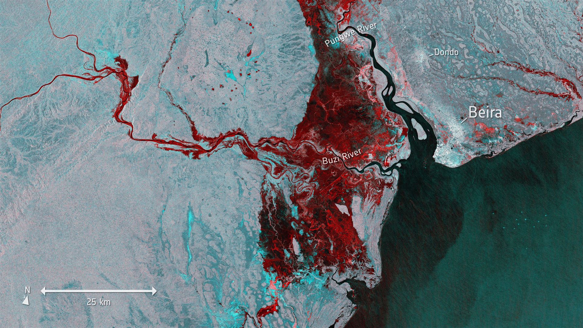
Sentinel-1 C-band SAR false-colour composite showing flood extent (red) around Beira, Mozambique, acquired 19 March 2019 following Cyclone Idai. Newly inundated areas are identified by the sharp drop in backscatter relative to the pre-event reference image — the operational NDFISAR method in action. Contains modified Copernicus Sentinel data (2019), processed by ESA — CC BY-SA 3.0 IGO.
2.6 Flood Potential Index (FPI)
The FPI is a composite operational index that integrates antecedent rainfall anomalies, current soil moisture state, and sometimes snowmelt contribution to produce a dynamically updated, spatially distributed estimate of flood generation potential. Unlike return-period quantiles (which describe statistical frequency) or FSI (which is static), the FPI is recalculated with every model cycle, making it suited to short-range operational flood monitoring and seasonal outlook communication.
Multiple implementations exist. The European Flood Awareness System (EFAS) combines the 30-day Standardized Precipitation Index with the soil saturation degree derived from the LISFLOOD model. NOAA's Climate Prediction Center expresses flood potential as ensemble streamflow percentile forecasts from its Ensemble Streamflow Prediction (ESP) system. A generalised formulation used in several academic and regional systems is:
SPIn = Standardized Precipitation Index at n-month accumulation window (typically 1–3 months)
Panom = current-period precipitation anomaly relative to climatological mean
w1, w2, w3 = weights summing to 1.0, calibrated regionally or by equal contribution
Output: continuous score or percentile class (below-normal / normal / above-normal / much-above-normal)
FPI values exceeding the 90th climatological percentile threshold flag catchments requiring heightened monitoring. For Africa, the FEWS NET seasonal monitoring platform uses an analogous composite — combining SPI anomaly with RFE2.0 rainfall departure — to flag elevated flood potential in key Sahelian and East African agricultural zones ahead of wet seasons.
2.7 Flood Susceptibility Index (FSI)
The FSI — also widely termed Flood Susceptibility Mapping (FSM) — characterises the intrinsic tendency of any landscape unit to be inundated, independent of the current hydrological state. It is a static spatial product derived entirely from terrain, soils, land use, and climatological data, without requiring real-time observations. FSI is most directly applicable to land-use planning, infrastructure siting, and community-level risk communication in data-scarce settings.
Typical conditioning factors and their directional influence on susceptibility:
- Elevation — negative correlation: lower-lying terrain more susceptible to inundation
- Slope — non-linear: very flat terrain accumulates water; moderate slopes funnel concentrated flow
- Topographic Wetness Index (TWI) — positive: high TWI areas have greater moisture accumulation potential (see section 2.10)
- Distance to river/channel — negative: proximity to the channel increases susceptibility
- Land use / land cover (LULC) — impervious surfaces > bare soil > cropland > forest
- Soil drainage class — poorly drained soils (Hydrologic Group C/D) markedly increase susceptibility
- Plan curvature — concave forms concentrate flow and promote water accumulation
- NDVI — negative: sparse vegetation → lower interception and infiltration → higher runoff generation
- Drainage density — high Dd → faster runoff concentration → heightened flash flood susceptibility
- Rainfall frequency index — areas with higher extreme rainfall climatology are more susceptible for given terrain
Derivation methods. Three broad approaches dominate the FSI literature:
- Multi-Criteria Decision Analysis (MCDA / AHP): Expert-assigned weights combined with pairwise comparison matrix (Saaty, 1980). Transparent and auditable but subjective; consistency ratio (CR < 0.1) required for valid AHP solutions. Widely used in Nigerian and Ethiopian flood susceptibility studies.
- Statistical bivariate methods: Frequency Ratio (FR) and Weight of Evidence (WoE) compute the statistical association between each conditioning factor class and historical flood inventory points. No calibration data volume requirement beyond the flood inventory itself.
- Machine learning classifiers: Random Forest, Gradient Boosting (XGBoost), Support Vector Machine (SVM), and deep learning (CNN) have dominated recent FSM publications. Using flood inventory points as training targets and conditioning factor rasters as features, these methods consistently achieve AUC > 0.90 in cross-validation. Tehrany et al. (2014) and Rahmati et al. (2016) are foundational references; Africa-specific studies include Njoku et al. (2023) for Nigeria and Abebe et al. (2022) for Ethiopia.
Output and validation. FSI maps are classified into five susceptibility classes — Very Low, Low, Moderate, High, Very High — and validated using Receiver Operating Characteristic (ROC) curves, the Area Under the Curve (AUC), and kappa coefficient against a withheld test inventory of historical flood occurrences.
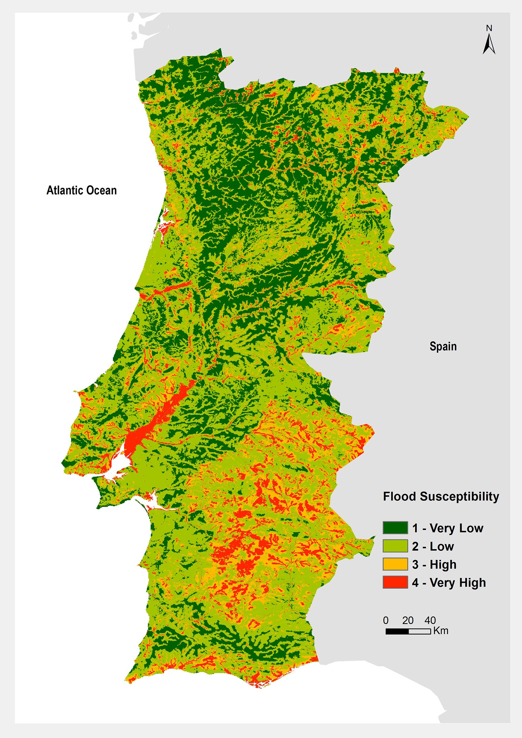
GIS-derived Flood Susceptibility Index map of mainland Portugal, classified from Very Low to Very High. Derived from terrain, soil, and climatic conditioning factors using a multi-criteria framework. Source: Jacinto et al. (2015), NHESS — CC BY 3.0.
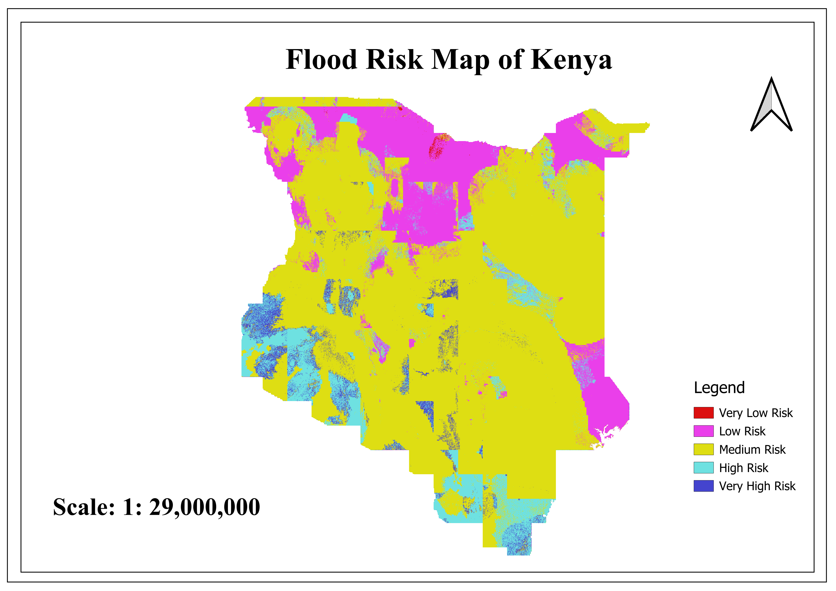
Flood risk classification map of Kenya showing five risk levels derived from composite spatial analysis. Africa-specific FSI products of this type are critical inputs for NDMA, county governments, and humanitarian pre-positioning. Source: Yakubu (2026) — CC BY 4.0.
2.8 Flood Vulnerability Index (FVI)
Flood hazard and susceptibility describe the physical system; vulnerability describes the human and built system's exposure and fragility. The FVI, formalised by Balica & Wright (2010) and Balica et al. (2012) for river and coastal flood systems, decomposes vulnerability into three dimensions — Social, Economic, and Physical/Environmental — each assessed through three lenses: Exposure (E), Susceptibility (S), and Resilience (R).
Sdim = Susceptibility sub-score — how easily can it be damaged or disrupted?
Rdim = Resilience sub-score — how effectively can the system absorb and recover?
Overall FVI = arithmetic or geometric mean of the three dimensional sub-indices, normalised to [0, 1]
Representative indicators for each component:
| Dimension | Exposure (E) | Susceptibility (S) | Resilience (R) |
|---|---|---|---|
| Social | Population density in flood zone; % living in poverty | % elderly (>65) + children (<5); literacy rate; flood awareness; disability prevalence | Early warning system reach; evacuation route quality; social safety nets; disaster preparedness |
| Economic | Value of assets in flood zone; % of GDP exposed; critical infrastructure count | Informal economy dependence; crop area in flood zone; uninsured asset ratio | GDP per capita; government fiscal space; private insurance coverage; access to credit |
| Physical / Environmental | Impervious surface %; elevation below flood level; proximity to water body | Building construction quality and age; drainage system capacity relative to design storm | Flood protection standard (design return period); green infrastructure retention; engineered storage capacity |
FVI is normalised so that 0 = zero vulnerability and 1 = maximum vulnerability. Cities or districts with FVI > 0.7 are considered at extreme vulnerability and are priority targets for flood risk reduction investment. The index has been applied to cities across South Asia, West Africa (Lagos, Accra), and East Africa (Nairobi, Dar es Salaam) in comparative studies.
INFORM Risk Index. The Index for Risk Management, developed by the EU Joint Research Centre (JRC) and published annually for all countries, applies a similar three-pillar structure to national-scale disaster risk:
V = Vulnerability pillar score (0–10): socioeconomic fragility + lack of coping capacity
CC−1 = inverse Coping Capacity score: institutional strength, DRR investment, early warning coverage
Geometric mean produces a balanced composite; scores available at drmkc.jrc.ec.europa.eu/inform-index
2.9 Flood Risk Index (FRI)
The FRI synthesises hazard, exposure, and vulnerability into a single composite score, operationalising the UNDRR/Sendai Framework risk equation. In quantitative terms, flood risk is most rigorously expressed as Expected Annual Damage (EAD):
f(Q) = probability density of annual peak discharge (derived from FFA)
Numerically approximated as: EAD ≈ Σ [D(Qi) × P(Qi)] across return period intervals
Units: USD/year or local currency/year; spatial aggregation gives EAD maps for portfolio risk
For comparative spatial assessments where monetary valuation is not available, a dimensionless FRI is computed:
Enorm = normalised exposure score (population, assets, infrastructure)
Vnorm = normalised vulnerability score (from FVI or proxy indicators)
CCnorm = normalised coping capacity (early warning, governance, DRR investment)
All components ∈ [0, 1]; FRI ∈ [0, 1] where 1 = maximum risk
Key operational FRI implementations and products:
- INFORM Risk Index (JRC/EC): annual country-level composite; flood sub-pillar within H&E component
- GFDRR/World Bank CCDR-Tools: open spatial risk toolkit for developing nations; gfdrr.github.io/CCDR-tools
- UNDRR Global Assessment Report (GAR): global flood risk exceedance curves; EAD estimates by country and basin
- FEMA HAZUS: US-specific multi-hazard risk model; EAD per census tract used for federal mitigation planning
- Swiss Re NATHAN / Munich Re NatCatSERVICE: proprietary global cat models underpinning (re)insurance pricing
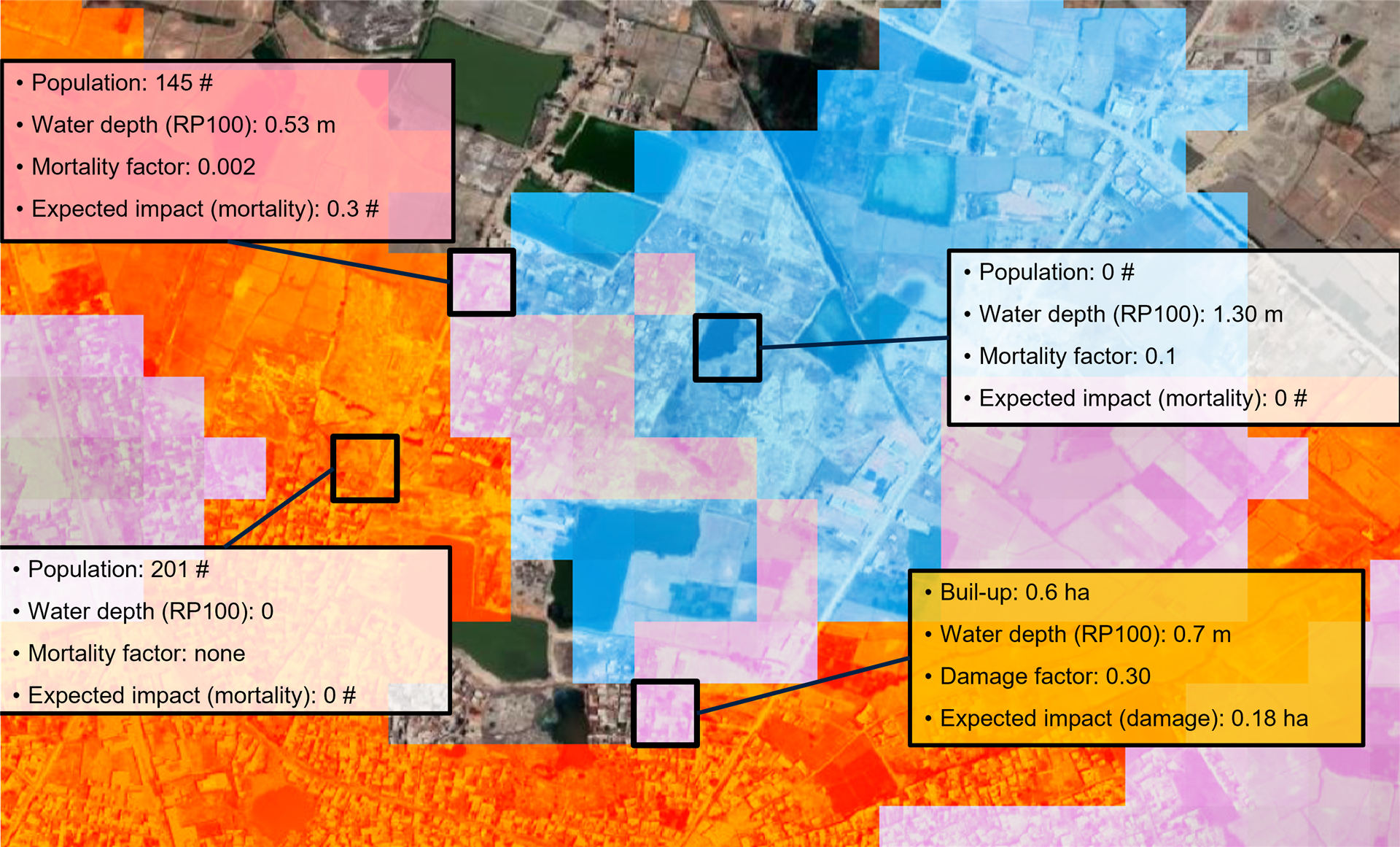
The GFDRR/World Bank spatial risk framework: hazard layer (flood depth-frequency from hydraulic modelling) intersected with exposure layer (gridded population and asset value) and vulnerability curves (depth-damage functions) to derive spatially explicit Expected Annual Damage estimates. This architecture underlies the FRI in most operational implementations. Source: Amadio M., GFDRR CCDR-Tools (2024) — World Bank Master Community Licence.
2.10 Morphometric Flood Indices
Basin morphometry provides a set of dimensionless shape and network parameters derived entirely from the DEM and extracted drainage network. These indices characterise how a catchment will respond to rainfall — its peak flow timing, magnitude, and attenuation — without requiring any streamflow observations. They are especially valuable for ungauged African basins where no streamflow record exists for statistical or model-based approaches.
The Topographic Wetness Index (TWI) — also called the Compound Topographic Index (CTI) — is the most widely used terrain-based flood susceptibility proxy:
β = local slope angle (radians); tan β → 0 on flat terrain → TWI → ∞ (maximum water accumulation)
High TWI (>10): topographic hollows, valley bottoms, floodplain margins — prime flood and soil saturation zones
Low TWI (<5): ridgelines, steep hillslopes — rapid drainage, low accumulation
Additional morphometric indices and their flood-response significance:
| Index | Formula | Flood Implication |
|---|---|---|
| Drainage Density (Dd) | Dd = ΣL / A (km/km²) | High Dd → efficient channel network → fast concentration → elevated peak flows |
| Stream Frequency (Fs) | Fs = N / A (streams/km²) | High Fs → dense network → flashy runoff response |
| Bifurcation Ratio (Rb) | Rb = Nu / Nu+1 | Low Rb (2–3): synchronous peaks, high flood hazard; High Rb (≥5): attenuated response |
| Circularity Ratio (Rc) | Rc = 4πA / P² | Rc → 1 (circular basin): synchronous flood peak; elongated (Rc → 0): delayed, attenuated peak |
| Form Factor (Ff) | Ff = A / Lb² | High Ff: compact basin → sharp concentrated peak; Low Ff: elongated → gradual response |
| Elongation Ratio (Re) | Re = (2/Lb)√(A/π) | Re → 1: circular, flood-prone; Re < 0.5: strongly elongated, flood-attenuated |
| Stream Power Index (SPI) | SPI = As × tan β | High SPI: erosive flow energy; identifies debris-flow and flood initiation zones |
| Relief Ratio (Rr) | Rr = H / Lb | High Rr: steep, rapid-response catchment with flashy hydrograph |
In GIS workflows, all these indices are computed from the filled and conditioned DEM using SAGA (QGIS), WhiteboxTools, or the ArcGIS Hydrology toolset. Morphometric-based flood susceptibility characterisation has been widely applied across Africa — Nigeria (Nwachukwu et al., 2020), Ethiopia (Markose & Jayappa, 2011), and the Nile Basin tributaries — typically combining multiple indices via AHP into a composite basin flood hazard score.
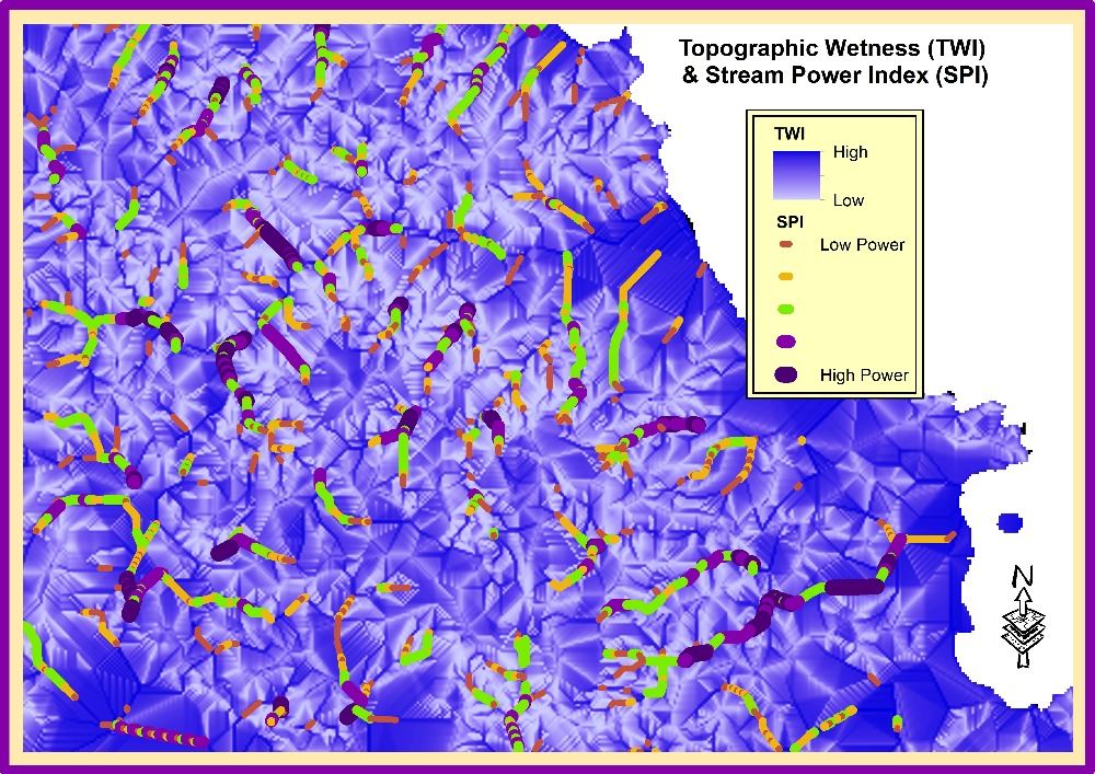
Topographic Wetness Index (TWI, left panel) and Stream Power Index (SPI, right panel) computed from a DEM for a Mediterranean catchment. High TWI values (warm colours) delineate valley bottoms, convergent hollows, and floodplain margins — the same terrain units that flood first and remain inundated longest. SPI identifies the highest-energy flow paths where erosion and rapid flood propagation occur. Source: Human & Physical Geography, European Science Photo Competition 2015 — CC BY-SA 4.0.
2.11 Compound Hazard Indices
Flood Hazard Index (FHI). A spatially explicit composite score combining flood frequency (return period exceedance probability), inundation depth, duration, and velocity, weighted by their damage-relevant contributions. Weights are derived through Analytic Hierarchy Process (AHP) or calibrated against historical damage records. FHI is used in urban planning, land-use zoning, and UNDRR/FEMA-style risk assessments.
Summary of principal flood indices.
| Index | Type | Time Scale | Data Required | Primary Use |
|---|---|---|---|---|
| QT (T-year quantile) | Statistical streamflow | Design/event | Long streamflow record | Infrastructure design, insurance |
| Flood Frequency Ratio | Statistical streamflow | Event | Streamflow record + Q̄ | RFFA, ungauged basins |
| BFI | Hydrograph-derived | Annual | Daily streamflow | Catchment characterisation |
| API | Rainfall proxy | Daily | Daily rainfall | Operational soil moisture state |
| SPI / SPEI | Rainfall statistical | Monthly (multi-scale) | Monthly rainfall ≥ 30 yr | Wet/dry monitoring, flood precursor |
| FFG | Flash flood threshold | 1–6 h (dynamic) | QPE, soil moisture, unit hydrograph | Flash flood early warning |
| FFPI | Static susceptibility | Climatological | DEM, soils, land cover | Flash flood zone mapping |
| SSI / SRI | Streamflow statistical | Monthly (multi-scale) | Monthly streamflow ≥ 30 yr | Hydrological flood/drought monitoring |
| SWI | Satellite soil moisture | Daily | SAR or passive microwave | Flood potential, model initialisation |
| FPI | Composite dynamic | Daily / weekly update | QPE, SPI, satellite soil moisture | Short-range flood potential monitoring; seasonal outlook communication |
| FSI | Static spatial susceptibility | Climatological | DEM, LULC, soils, drainage network | Land-use planning, infrastructure siting, community risk mapping |
| FVI | Socio-economic vulnerability | Annual / census cycle | Population, assets, governance indicators | Risk reduction prioritisation; humanitarian pre-positioning |
| FRI / EAD | Composite risk | Annual exceedance | Hazard maps + exposure + damage functions | National risk accounting; cat modelling; DRR investment prioritisation |
| TWI | Terrain morphometric | Climatological | DEM (filled, conditioned) | Soil moisture proxying; FSI conditioning factor; ungauged basin characterisation |
| Dd, Rb, Rc, Ff | Basin morphometric | Climatological | DEM + stream network extraction | Ungauged basin flash flood response characterisation |
| MNDWI / AWEI | Optical remote sensing | Days–weeks (cloud-limited) | Multispectral imagery | Post-event inundation mapping |
| NDFISAR | SAR remote sensing | Hours–days | Sentinel-1 pre/post scenes | Cloud-independent flood mapping |
| FHI | Compound hazard composite | Climatological | Multiple spatial layers | Risk zoning, urban planning |
3. Deriving Flood Indices: Key Methods
3.1 Flood Frequency Analysis
FFA is the statistical backbone for all return-period flood indices. The workflow involves assembling an extreme-flow series, fitting a probability distribution, and estimating quantiles at desired return periods.
-
Assemble the data series Extract the Annual Maximum Series (AMS: one peak per year) or Peaks-Over-Threshold (POT: all peaks above a threshold). POT uses more data and is statistically efficient for short records; AMS is the standard for infrastructure design. Minimum record length: 20 years (WMO guidance), with ≥ 30 years strongly preferred for reliable quantile estimation beyond the 50-year return period.
-
Estimate distribution parameters via L-moments L-moments (Hosking, 1990) are linear combinations of order statistics, more robust to outliers than conventional product moments. They are the recommended estimation method for short records (n < 50), mandated by the UK Flood Estimation Handbook (Robson & Reed, 1999), and preferred internationally. L-moment ratios (L-CV, L-skewness, L-kurtosis) discriminate between candidate distributions via goodness-of-fit tests such as the Z-test of Hosking & Wallis (1997).
-
Select the best-fit distribution For global and pan-African applications, the GEV is generally preferred for its flexibility. In the US, LP3 with log-space moments is mandated by Bulletin 17C (England et al., 2019). The Gumbel (EV1) — GEV with ξ = 0 — is adequate for moderate samples but systematically underestimates heavy-tailed quantiles common in tropical and semi-arid African catchments.
-
Regional FFA for ungauged basins The index flood method (Dalrymple, 1960) assumes normalised quantiles QT/Q̄ are homogeneous within a hydrological region. Regional growth curves are estimated from pooled gauged data and applied to ungauged sites via regression equations relating Q̄ to catchment descriptors (area, mean annual rainfall, soil permeability, slope). This underpins QMED estimation in the FEH and analogous regional methods across Africa. For most African countries, this remains the only viable path to design flood estimation.
Non-stationarity: Classical FFA assumes flood series are statistically stationary — that the underlying probability distribution is not changing over time. Rapid urbanisation and land-use change violate this assumption across many African catchments. Non-stationary FFA methods allowing distribution parameters to trend with time or climate covariates (Villarini et al., 2009) are increasingly recommended for long-term infrastructure design in regions undergoing rapid change.
3.2 Flash Flood Guidance Derivation
The FFG computational framework (Sweeney, 1992; Carpenter et al., 1999) derives a dynamic rainfall threshold from real-time soil moisture state and catchment unit hydrograph properties.
-
Continuous soil moisture accounting A soil moisture accounting model (SAC-SMA in GFFGS implementations) tracks water contents of multiple soil layers in near-real-time, updated with each QPE increment. The current state defines the antecedent soil moisture deficit for each basin — the additional water storage available before saturation-excess runoff begins.
-
Threshold runoff volume For each storm duration τ (typically 1, 3, and 6 hours), the threshold runoff volume Qthresh(τ) that would produce bankfull discharge at the basin outlet is computed using the derived unit hydrograph and channel routing. This is the critical link between basin hydraulics and the rainfall threshold.
-
Derive FFG(τ) FFG(τ) = threshold runoff volume + current soil moisture deficit, expressed as a spatially averaged rainfall depth over the basin. As soils wet up, the deficit shrinks and FFG falls — heightening alert sensitivity in real time. Drier basins have higher FFG (more rainfall required to cause flooding); saturated basins may have FFG near zero.
-
Operational comparison with QPE/QPF Real-time QPE from satellite (CMORPH, PERSIANN-CCS in AfFFGS) is aggregated over τ and spatially compared to FFG maps. Where QPE > FFG, a flash flood threat is flagged for downstream locations. QPF from NWP models extends the comparison to future periods for forecast lead time.
3.3 SPI and SSI Computation
Both SPI and SSI follow the same framework applied to precipitation and streamflow respectively. The standard steps are: (1) assemble a historical monthly time series of at least 30 years; (2) fit a two-parameter gamma distribution (SPI) or Pearson Type III (SSI) to the accumulation-window data; (3) transform cumulative probability to standard normal via the equiprobability transformation SPI = Φ−1(Fgamma(x)), where Φ−1 is the inverse standard normal CDF. The resulting values are universally interpretable: ±0 = median conditions; ±1.5 = severely wet/dry; ±2.0 = extreme conditions. Computation is available in the WMO SPI Tool and multiple open-source Python/R libraries (e.g. the climate-indices Python package).
3.4 SAR Flood Mapping Workflow
Operationally, SAR flood mapping uses Sentinel-1 IW (Interferometric Wide Swath) GRD products at 10 m, freely available through the Copernicus Open Access Hub or Google Earth Engine. The standard pipeline:
- Download and radiometrically calibrate pre-event and co-event scenes (ESA SNAP toolbox or GEE).
- Apply terrain correction using the Copernicus DEM GLO-30.
- Convert to decibels; compute the difference image: Δσ° = σ°post[dB] − σ°pre[dB].
- Threshold: Δσ° < −3 to −5 dB typically identifies newly inundated areas (Boni et al., 2016).
- Apply ancillary masks to suppress false positives: urban radar shadow, permanent water bodies, slopes >5°.
- Vectorise and deliver flood polygon as a GIS layer.
This workflow underpins Copernicus EMS Rapid Mapping, UNOSAT flood response products, and SERVIR-Africa flood mapping. Google Earth Engine makes the entire pipeline executable at continental scale without local data downloads.
4. Operational Applications of Flood Indices
4.1 Real-Time Early Warning
Flood early warning systems integrate multiple indices in a tiered pipeline. The sequence typically proceeds: QPE compared against FFG thresholds for flash flood guidance at sub-daily timescales → short-range NWP precipitation driving a hydrological model for river-reach flood warnings at 1–5 day lead → ensemble forecast streamflow compared against Q2yr/Q5yr/Q20yr thresholds to classify alert levels (yellow/orange/red) → SWI and API used to adjust threshold sensitivity under wet antecedent conditions. The WMO recommends a four-tier alert scheme (advisory → watch → warning → emergency) anchored to specific return period exceedances, communicated to national disaster management authorities through standardised products.
4.2 Flood Inundation Mapping for Emergency Response
Within 12–24 hours of a major flood event, MNDWI, AWEI, and SAR-derived flood extents are produced by Copernicus EMS, UNOSAT, and SERVIR. These products provide affected-area estimates for evacuation guidance, relief logistics, and damage assessment. Post-event comparison of observed inundation to hydraulic model predictions (HEC-RAS 2D, LISFLOOD-FP) validates and updates national flood hazard maps.
4.3 Insurance and Catastrophe Modelling
The (re)insurance industry uses QT and FHI as primary inputs to catastrophe (cat) models. Annual average loss (AAL) is calculated by integrating depth-damage functions over the full frequency distribution of flood events. Index-based parametric insurance — using satellite rainfall or flood extent indices as automatic payment triggers — is being piloted for smallholder agriculture in Africa, avoiding the claims adjustment bottleneck that undermines traditional indemnity insurance in low-capacity settings.
4.4 Infrastructure Design and Climate Adaptation
Design floods for hydraulic infrastructure are QT values chosen to balance capital cost and residual risk. Climate change adaptation requires stress-testing designs under non-stationary conditions: CMIP6 downscaled precipitation products allow practitioners to evaluate how Q50 or Q100 estimates shift under mid- and end-century warming scenarios. The key emerging concept is design life risk — the probability of at least one exceedance over the infrastructure's service lifetime — which rises as the underlying frequency distribution shifts.
5. Global Flood Forecasting Systems
5.1 Global Platforms
Global Flood Awareness System (GloFAS). Developed by ECMWF and the EU Joint Research Centre (JRC), GloFAS has been operational since 2011 and became a Copernicus Emergency Management Service in 2018. It uses ECMWF's 51-member ensemble prediction system (ENS) as atmospheric forcing, driving the LISFLOOD hydrological-routing model (De Roo et al., 2000) at approximately 0.1° (~10 km) over a global river network derived from the MERIT DEM. Ten-day ensemble streamflow forecasts are expressed as exceedance percentiles relative to climatological simulations; alert thresholds correspond to the 2-year (yellow), 5-year (orange), and 20-year (red) return period equivalents. GloFAS-Seasonal extends this to four-month probabilistic streamflow outlooks using ECMWF SEAS5 forcing. The Alfieri et al. (2013) paper describes the original system; Emerton et al. (2016) provide a broader review. Live platform: globalfloods.eu.
Global Flood Monitoring System (GFMS). Operated by the University of Maryland with NASA support, GFMS provides near-real-time (≈4-hour latency) global flood detection and streamflow estimates using GPM IMERG satellite precipitation to force the Variable Infiltration Capacity (VIC) land surface model at 1/8° (~12 km) resolution (Wu et al., 2014). Unlike GloFAS's ensemble-forecast approach, GFMS is primarily a monitoring and detection system — flagging where active flooding is occurring based on current streamflow exceeding climatological thresholds. Products include gridded streamflow, flood detection maps, and inundation depth estimates. Products are accessible through NASA Earthdata Disasters portal and the GFMS research team at UMD.
WMO Global Flash Flood Guidance System (GFFGS). The WMO GFFGS programme has established regional FFGS implementations covering South Asia, Southeast Asia, the Middle East, Central America and the Caribbean, and sub-Saharan Africa (AfFFGS). Each regional system uses the SAC-SMA soil moisture accounting model, basin-level unit hydrographs, and 6-hourly QPE from satellite to produce FFG thresholds for tens of thousands of small basins. AfFFGS covers over 40 African countries and disseminates products to National Meteorological and Hydrological Services (NMHSs) for local early warning activation. Details at wmo.int/ffgs.
Dartmouth Flood Observatory (DFO). The DFO maintains a global archive of large flood events detected from MODIS, Sentinel-1, Landsat, and supplemented by news and government reports, extending back to 1985. The database is invaluable for historical flood frequency analysis, benchmarking forecast systems, and identifying long-term trends. Available at floodobservatory.colorado.edu.
5.2 Africa-Focused Systems
FEWS NET (Famine Early Warning Systems Network). USAID's FEWS NET is the primary operational food security and humanitarian early warning network for sub-Saharan Africa, the Greater Horn, Central America, and other crisis-prone regions. Its hydrological monitoring component integrates near-real-time satellite rainfall (RFE2.0, CHIRPS), NDVI anomalies, SPI, and streamflow anomalies into monthly food security outlooks. FEWS NET also produces seasonal hydrological assessments highlighting flood risk for key agricultural and pastoralist regions. All products freely available at fews.net.
African Flood and Drought Monitor (AFDM). Developed at Princeton University (Sheffield et al., 2014), the AFDM uses the VIC land surface model at 0.25° resolution, forced by a combination of gauge observations, satellite data, and reanalysis, to generate daily soil moisture, runoff, streamflow anomaly, and standardised index (SSI, SRI) estimates for all of Africa. Historical simulations extend to 1950 via the Princeton Global Forcing dataset, providing the climatological baseline required for anomaly computation. Now hosted at Cornell University's Earth and Atmospheric Sciences department.
SERVIR-Africa. SERVIR is a joint NASA–USAID programme providing satellite-derived Earth observation services for development decisions. The SERVIR Eastern and Southern Africa hub (hosted at RCMRD, Nairobi) and SERVIR West Africa node support flood mapping, seasonal outlooks, and hydrological drought monitoring using MODIS, Sentinel-1, and Landsat products. SAR-based flood extent maps are routinely shared with disaster management authorities in East Africa within 24–48 hours of major events. Details at servirglobal.net.
Copernicus Emergency Management Service (CEMS) — Rapid Mapping. CEMS activates on-demand Rapid Mapping globally within 12–24 hours of a disaster, including floods across Africa. SAR-based flood extent from Sentinel-1 is the primary product, supplemented by commercial VHR optical imagery. Notable African activations include Cyclone Idai in Mozambique (2019), Sudan annual Nile floods, Nigeria's Niger/Benue confluence flooding, and recurring East Africa flash floods. Products are publicly available at emergency.copernicus.eu.
5.3 National Capacities in Africa
| Country / Region | Key Institution(s) | Capability |
|---|---|---|
| Nigeria | NIHSA, NiMet | Annual Flood Outlook (NIHSA); seasonal ENSO-based rainfall forecasts; coordination with AfFFGS; NEWMAP gauge modernisation programme |
| South Africa | SAWS, DWS, WRC | Most advanced NMHS in Africa; national weather radar network; NWP (UM); real-time river gauging; operational flood warnings for major basins |
| Ethiopia | MoWIE, EMI | Major reservoir operations; Nile Basin Initiative cooperation; NWP-driven seasonal flood outlooks |
| East Africa (regional) | ICPAC (IGAD Centre) | Greater Horn of Africa Consensus Outlook (GHACOF); ENSO-linked seasonal rainfall and flood risk forecasts; capacity building |
| West Africa (regional) | ACMAD, PRESAO | West Africa seasonal rainfall outlook (PRESAO); WMO SWFDP NWP guidance relay to NMHSs |
| Southern Africa (regional) | SARCOF, SADC-HYCOS | Seasonal consensus rainfall forecasts; Zambezi/Limpopo transboundary gauge network |
| Pan-Africa | TAHMO | Deploying 1,000 low-cost automated weather stations; ~800 operational by 2025; addresses critical gauge gap |
6. Rainfall Forecasting by Temporal Scale
6.1 Nowcasting (0–6 Hours)
At very short lead times, NWP models cannot respond faster than convective initiation timescales. Radar-based extrapolation dominates. The STEPS (Short-Term Ensemble Prediction System) framework (Seed et al., 2004; Bowler et al., 2006) uses optical flow algorithms to extrapolate radar echoes forward in time while applying stochastic perturbation to generate probabilistic ensembles that account for forecast uncertainty. The open-source PySTEPS library provides a community implementation now used by NMHSs across Europe, Australasia, and a growing number in the Global South.
Deep learning nowcasting has produced state-of-the-art results: DeepMind's DGMR (Ravuri et al., 2021) and Google's MetNet-3 (Andrychowicz et al., 2023) outperform STEPS-type methods on standard benchmarks at lead times up to 6–8 hours. These models are entering operational testing at major NMHSs.
Africa constraint: C-band weather radar remains sparse across sub-Saharan Africa. South Africa (SAWS) operates a national network; Kenya, Nigeria, Ethiopia, and a handful of others have partial coverage. Most of the continent relies on satellite QPE for sub-hourly rainfall monitoring, which lacks the resolution and latency for true flash flood nowcasting. This gap makes satellite-based FFG (AfFFGS) the de facto flash flood warning mechanism across most of Africa.
6.2 Short-Range (6–72 Hours)
Global and limited-area NWP models dominate at 6–72 hours. Key deterministic products:
- ECMWF HRES (9 km global, 10-day): consistently the best-verified global NWP model; used by over 130 NMHSs worldwide.
- NOAA GFS (13 km global, 16-day): freely available via NOMADS; widely used by African NMHSs without ECMWF data access.
- UK Met Office UM (10 km global, 7-day): used by Commonwealth NMHSs in Africa via UKMO partnership agreements.
- WRF (Weather Research and Forecasting Model): community mesoscale NWP; routinely nested to 1–5 km over target regions; widely used in African research and some operational contexts, including at South African Weather Service and several university-based research groups.
Ensemble NWP is essential for probabilistic flood forecasting. The ECMWF ENS (51 members, 18 km, 15-day) and NOAA GEFS (31 members, 13 km, 16-day) provide the uncertainty characterisation needed to drive ensemble hydrological models and probabilistic alert products. The WMO SWFDP (Severe Weather Forecasting Programme) distils global NWP guidance for delivery to African NMHSs that lack indigenous NWP capability.
6.3 Medium-Range (3–14 Days)
ECMWF ENS dominates skill at medium range globally and is the primary meteorological forcing for GloFAS 10-day flood forecasts. Systematic biases in NWP rainfall must be corrected before hydrological model forcing: BCSD (Bias Correction Spatial Disaggregation) (Wood et al., 2002) and quantile mapping are standard preprocessing steps. The TIGGE archive (Bougeault et al., 2010), hosted at ECMWF, provides harmonised multi-model ensemble forecasts from 10 global centres, enabling research into multi-model ensemble flood forecasting approaches that reduce single-model structural uncertainty.
6.4 Seasonal (1–6 Months)
Seasonal flood outlooks are built on coupled ocean-atmosphere GCMs that capture dominant forcing from ENSO, the Indian Ocean Dipole (IOD), and the Madden-Julian Oscillation (MJO). Key products for Africa:
- ECMWF SEAS5 (51-member, 7-month): state-of-the-art coupled GCM; drives GloFAS-Seasonal for long-range river flow outlooks; best overall skill globally.
- NOAA CFSv2 (24-member): freely available; widely used as a base for WMO regional outlook forums across Africa.
- IRI Seasonal Forecasts (Columbia University): synthesises multi-model seasonal forecasts with particular focus on Africa and food security; probabilistic rainfall anomaly maps for 3-month seasons at iri.columbia.edu.
- ICPAC GHACOF: Greater Horn of Africa Consensus Outlook Forum; produces tri-seasonal probabilistic rainfall forecasts for East Africa using ENSO-based statistical and GCM methods, critical for pre-positioning humanitarian flood response.
- SARCOF: Southern Africa Regional Climate Outlook Forum; ENSO-informed seasonal consensus for the October–December and January–March seasons covering the Zambezi and Limpopo flood seasons.
- PRESAO: West Africa seasonal rainfall outlook coordinated by ACMAD; essential for anticipating Niger and Volta basin flooding and Sahel flash flood seasons.
6.5 Satellite QPE for Africa
The sparse and declining rain gauge network in Africa makes satellite Quantitative Precipitation Estimation (QPE) the operational backbone for rainfall monitoring and hydrological model forcing. Principal products:
| Product | Provider | Resolution | Latency | Record | Africa Strength |
|---|---|---|---|---|---|
| GPM IMERG | NASA / JAXA | 0.1°, 30-min | ~4 h (Early/Late) | 2000–present | Best global QPE; merges active DPR + passive microwave; gauge-calibrated Final run |
| CHIRPS | UCSB CHC / USAID | 0.05°, daily | ~3 weeks (Final) | 1981–present | Long record; bias-corrected against CHPclim; ideal for FFA and trend analysis |
| TAMSAT | University of Reading | 0.0375°, daily | Near real-time | 1983–present | Africa-specific CCD + gauge blending; best-verified product for sub-Saharan Africa |
| CMORPH | NOAA CPC | 0.072°, 30-min | ~1 h | 2002–present | Fast morphing of passive microwave retrievals; good for operational near-RT monitoring |
| RFE2.0 | NOAA CPC / FEWS NET | 0.1°, daily | ~1 day | 2001–present | Purpose-built for Africa; integrates GTS gauge reports; standard FEWS NET product |
| PERSIANN-CCS | UCI / CHRS | 0.04°, hourly | ~1 h | 2003–present | Highest spatial resolution; captures convective detail; primary QPE input to AfFFGS |
7. Streamflow and Discharge Forecasting Methods
7.1 Lumped Conceptual Models
Conceptual models represent basin-scale water stores as simplified linked reservoirs with empirical transfer functions. Despite their simplicity, they remain operational workhorses because of computational efficiency, ease of calibration, and robust performance across diverse climates.
- HBV (Bergström, 1976): 14–20 parameters; snow + soil moisture + response + routing routines; widely used in Scandinavia and across Africa via HBV-Light. Parameter parsimony makes it well-suited to data-scarce African settings.
- SAC-SMA (Burnash et al., 1973): NOAA/NWS operational model since the 1970s; 16-parameter soil moisture accounting; coupled with kinematic wave routing in the US National Water Model; provides the soil moisture backbone of the GFFGS.
- GR4J (Perrin et al., 2003): 4-parameter daily model developed by INRAE (France); extensively calibrated across West and Central Africa by the former ORSTOM/IRD network; consistently strong performance on tropical and Sahelian catchments with short records.
- TOPMODEL (Beven & Kirkby, 1979): topographic wetness index-based variable contributing area concept; best suited to humid, topographically complex catchments; less applicable in semi-arid African settings where Hortonian overland flow dominates.
7.2 Distributed and Semi-Distributed Models
Distributed models subdivide catchments into spatial units (subcatchments, grid cells, hydrological response units) to represent spatial variability in land use, soils, and topography explicitly.
- SWAT (Arnold et al., 1998): ArcSWAT and QSWAT interfaces; among the most widely applied hydrological models globally, with over 500 published Africa applications; semi-distributed; excellent for water resources management and land-use change impact assessment. Available at swat.tamu.edu.
- VIC (Liang et al., 1994): full energy and water balance at each grid cell; standard 0.25° global configuration backs both GFMS (NASA) and the African Flood and Drought Monitor; captures snow, frozen soil, and multi-layer energy exchange — less commonly needed in tropical Africa but important at high elevations.
- LISFLOOD (De Roo et al., 2000): PCRaster-based distributed model developed by JRC; powers GloFAS globally at 0.1°; includes snowmelt, lake and reservoir routing, and floodplain inundation modules.
- mHM (mesoscale Hydrological Model) (Samaniego et al., 2010): uses Multiscale Parameter Regionalization (MPR) to derive model parameters from readily available soil and geology maps without basin-specific calibration — particularly valuable for ungauged African basins. Available at mhm-ufz.org.
7.3 Ensemble Streamflow Prediction (ESP)
ESP (Day, 1985) is a probabilistic extended-range technique in which the hydrological model is initialised from current observed states and driven by an ensemble of historical meteorological sequences sampled from the observed archive. Each historical year serves as an equiprobable scenario for future weather; ensemble spread captures seasonal climate uncertainty. ESP is used by NOAA/NWS River Forecast Centers for 2–6 week probabilistic forecasts and is particularly effective for reservoir operations planning. When ENSO state is known, historical years can be stratified by phase (El Niño/La Niña/neutral), improving skill in ENSO-sensitive regions of Africa including the Greater Horn, Southern Africa, and West Africa Sahel (Hamlet & Lettenmaier, 1999).
7.4 Machine Learning and Deep Learning
ML approaches for streamflow forecasting have advanced rapidly. Key developments:
- LSTM networks (Kratzert et al., 2018, 2019): Long Short-Term Memory recurrent networks with explicit memory cells that learn temporal rainfall-runoff dynamics without imposed physical structure. A single LSTM trained on 531 US basins — without basin-specific calibration — outperformed individually calibrated HBV on median Nash-Sutcliffe Efficiency. The approach shows strong potential for ungauged African catchments via transfer learning.
- Transformer architectures: encoder-decoder transformers (attention mechanisms) extend LSTM performance at longer lead times and are an active research frontier for multi-basin global prediction.
- Random forests and gradient boosting: effective for peak flow regression and flash flood binary classification, with interpretability advantages and lower data requirements.
- Physics-informed ML (PIML): hybrid frameworks embedding physical constraints (water balance closure, mass conservation) into the neural network loss function, improving extrapolation to extreme events outside the training distribution — critical for flood applications.
ML in Africa — caveats: Supervised ML models require long, high-quality training records. The sparse and discontinuous gauge record across much of Africa undermines purely data-driven approaches. Hybrid physics-ML models, pre-training on data-rich regions with fine-tuning on short African records, and uncertainty-aware ensemble frameworks are the active frontiers for improving ML applicability in low-data contexts.
7.5 Data Assimilation
Data assimilation (DA) updates model state variables in real time as new observations arrive, reducing initialisation error and improving short-lead forecast accuracy. The Ensemble Kalman Filter (EnKF) is the most widely used DA technique in operational hydrology, updating soil moisture, snow water equivalent, and channel storage states using streamflow gauge observations. For Africa, satellite-derived observations are particularly valuable DA inputs: SMAP and ASCAT surface soil moisture, GRACE-FO terrestrial water storage anomalies, and river stage from Sentinel-3 radar altimetry are all being assimilated into continental and global hydrological models to compensate for declining ground-based observation density (Wanders et al., 2014).
8. Challenges and the Path Forward in Africa
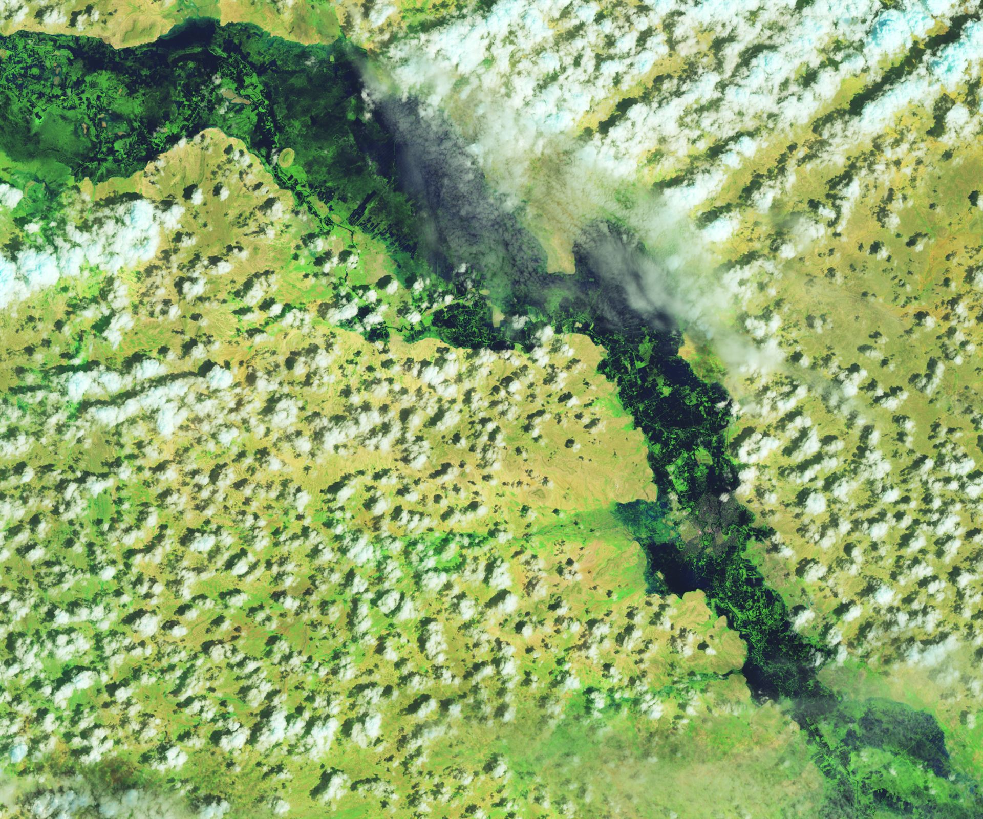
Landsat 8 OLI false-colour composite showing catastrophic flooding in Somalia (November 2023), one of the most severe flood events in East Africa in decades. Flooded areas appear in blue against brown dry land. Events like this — driven by the exceptional 2023 IOD positive phase — underscore the need for operational seasonal outlooks and robust early warning infrastructure that the continent still largely lacks. Image: NASA Earth Observatory / Lauren Dauphin (USGS Landsat data) — public domain.
8.1 The Gauge Network Crisis
A 2012 WMO assessment documented that the density of hydrometric stations across Africa fell by 40–80% between 1980 and 2010 in many sub-regions, driven by funding constraints, equipment deterioration, civil conflict, and institutional fragmentation. This is the single largest obstacle to operational flood forecasting in Africa: without real-time streamflow observations for model updating and verification, forecast skill degrades and cannot be systematically evaluated. Two complementary responses: TAHMO is deploying ~1,000 low-cost internet-connected automatic weather stations across sub-Saharan Africa; and satellite-based streamflow estimation from radar altimetry (Sentinel-3, SWOT) and ML-based discharge rating curves offer paths to real-time data at ungauged reaches.
8.2 Ungauged Basin Problem
The IAHS PUB (Predictions in Ungauged Basins) initiative (Sivapalan et al., 2003; Hrachowitz et al., 2013) produced a decade of advances in predicting flood responses without gauge data. For Africa, dominant approaches are: spatial proximity (donor catchment analogy), parameter regionalisation via catchment descriptors (mHM's MPR method), and regionalised flood frequency growth curves. Pre-trained global LSTM models (Gauch et al., 2021) offer a promising newer path — their cross-basin training on data-rich regions can be transferred to ungauged African basins with limited fine-tuning data.
8.3 Urban Flash Flooding
West and East Africa's rapidly growing cities — Lagos, Kano, Accra, Nairobi, Dar es Salaam, Kinshasa — face intensifying flash flood hazard as impervious cover increases faster than drainage infrastructure is upgraded. Urban hydrology requires sub-km spatial resolution that global forecast systems cannot meet. City-scale hydrodynamic models (SWMM, InfoWorks ICM, MIKE FLOOD) need to be coupled to NWP through spatial downscaling, and AfFFGS's rural-basin FFG framework requires a separate urban flash flood component. This is an urgent unmet need across virtually every major African city.
8.4 Transboundary Coordination
Africa's major flood systems are transboundary: the Niger, Nile, Zambezi, Congo, Volta, and Senegal all cross multiple national jurisdictions. Effective early warning requires real-time data sharing across borders and coordinated reservoir operations. The WMO HYCOS sub-basin networks — NIGER-HYCOS, VOLTA-HYCOS, CONGO-HYCOS, ZAMBEZI-HYCOS — provide frameworks for transboundary hydrometric data exchange, though operational continuity varies considerably across network nodes.
9. Conclusion
Flood indices provide the quantitative language through which flood hazard is described, communicated, and acted upon. No single index is sufficient: QT quantiles serve infrastructure design; FFG drives real-time flash flood warning; SPI and SSI track multi-scale wetness conditions; SAR-derived NDFI maps inundation rapidly and objectively under cloud cover. Operational forecasting systems stitch these indices together across temporal scales — from the nowcast (radar, deep learning) through medium-range ensemble hydrological forecasting (GloFAS, GFMS) to seasonal outlooks (GloFAS-Seasonal, ICPAC, SARCOF).
For Africa, the gap between the sophistication of available methods and their operational deployment remains large. The root constraints — sparse ground observation networks, limited institutional capacity, and fragmented transboundary data sharing — are not technical but organisational and financial. The tools described in this article, most of them freely available, provide a credible path to substantially improved flood early warning across the continent. The investment needed is not primarily in developing new science but in deploying, maintaining, and building local capacity around what already exists.
10. References
- Alfieri, L., Burek, P., Dutra, E., Krzeminski, B., Muraro, D., Thielen, J., & Pappenberger, F. (2013). GloFAS — global ensemble streamflow forecasting and flood early warning. Natural Hazards and Earth System Sciences, 13(3), 777–787. doi:10.5194/nhess-13-777-2013
- Abebe, W. B., Biru, M. M., Asfaw, T. G., & Gezie, A. A. (2022). Flood susceptibility mapping using GIS-based multi-criteria evaluation and machine learning models in the Ketar watershed, Ethiopia. Geoenvironmental Disasters, 9(1), 1–20. doi:10.1186/s40677-022-00196-0
- Albergel, C., Rüdiger, C., Pellarin, T., et al. (2008). From near-surface to root-zone soil moisture using an exponential filter. Hydrology and Earth System Sciences, 12(6), 1323–1337. doi:10.5194/hess-12-1323-2008
- Arnold, J. G., Srinivasan, R., Muttiah, R. S., & Williams, J. R. (1998). Large area hydrologic modelling and assessment. Journal of the American Water Resources Association, 34(1), 73–89. doi:10.1111/j.1752-1688.1998.tb05961.x
- Bergström, S. (1976). Development and application of a conceptual runoff model for Scandinavian catchments. SMHI Report RHO 7, Norrköping.
- Beven, K. J., & Kirkby, M. J. (1979). A physically based, variable contributing area model of basin hydrology. Hydrological Sciences Bulletin, 24(1), 43–69. doi:10.1080/02626667909491834
- Balica, S. F., & Wright, N. G. (2010). Reducing the complexity of the flood vulnerability index. Environmental Hazards, 9(4), 321–339. doi:10.3763/ehaz.2010.0043
- Balica, S. F., Wright, N. G., & van der Meulen, F. (2012). A flood vulnerability index for coastal cities and its use in assessing climate change impacts. Natural Hazards, 64(1), 73–105. doi:10.1007/s11069-012-0234-1
- Boni, G., Ferraris, L., Pulvirenti, L., et al. (2016). A prototype system for flood monitoring based on flood forecast combined with SAR imagery. IEEE Journal of Selected Topics in Applied Earth Observations and Remote Sensing, 9(6), 2794–2805. doi:10.1109/JSTARS.2016.2514402
- Boorman, D. B., Hollis, J. M., & Lilly, A. (1995). Hydrology of soil types: a hydrologically-based classification of the soils of the United Kingdom. Institute of Hydrology Report 126, Wallingford.
- Bowler, N. E., Pierce, C. E., & Seed, A. W. (2006). STEPS: A probabilistic precipitation forecasting scheme which merges an extrapolation nowcast with downscaled NWP. Quarterly Journal of the Royal Meteorological Society, 132(620), 2127–2155. doi:10.1256/qj.04.100
- Burnash, R. J. C., Ferral, R. L., & McGuire, R. A. (1973). A generalized streamflow simulation system: Conceptual modeling for digital computers. Joint Federal-State River Forecast Center, Sacramento.
- Carpenter, T. M., Georgakakos, K. P., & Sperfslage, J. A. (1999). On the parametric and NEXRAD-radar sensitivities of a distributed hydrologic model suitable for operational use. Journal of Hydrology, 253, 169–193.
- Chapman, T. (1999). A comparison of algorithms for stream flow recession and baseflow separation. Hydrological Processes, 13(5), 701–714. doi:10.1002/HYP.774
- Dalrymple, T. (1960). Flood frequency analyses. USGS Water Supply Paper 1543-A, US Geological Survey, Reston.
- Day, G. N. (1985). Extended streamflow forecasting using NWSRFS. Journal of Water Resources Planning and Management, 111(2), 157–170. doi:10.1061/ASCE.0733-9496
- De Roo, A. P. J., Wesseling, C. G., & Van Deursen, W. P. A. (2000). Physically based river basin modelling within a GIS: The LISFLOOD model. Hydrological Processes, 14(11–12), 1981–1992. doi:10.1002/HYP.49
- Emerton, R. E., Stephens, E. M., Pappenberger, F., et al. (2016). Continental and global scale flood forecasting systems. WIREs Water, 3(3), 391–418. doi:10.1002/wat2.1137
- England, J. F., Cohn, T. A., Faber, B. A., et al. (2019). Guidelines for Determining Flood Flow Frequency — Bulletin 17C. USGS Techniques and Methods 4-B5. doi:10.3133/tm4B5
- Feyisa, G. L., Meilby, H., Fensholt, R., & Proud, S. R. (2014). Automated Water Extraction Index: A new technique for surface water mapping using Landsat imagery. Remote Sensing of Environment, 140, 23–35. doi:10.1016/j.rse.2013.08.029
- Funk, C., Peterson, P., Landsfeld, M., et al. (2015). The Climate Hazards Infrared Precipitation with Stations — a new environmental record for monitoring extremes. Scientific Data, 2, 150066. doi:10.1038/sdata.2015.66
- Gauch, M., Kratzert, F., Klotz, D., et al. (2021). Rainfall–runoff prediction at multiple timescales with a single Long Short-Term Memory network. Hydrology and Earth System Sciences, 25(4), 2045–2062. doi:10.5194/hess-25-2045-2021
- Hamlet, A. F., & Lettenmaier, D. P. (1999). Columbia River streamflow forecasting based on ENSO and PDO climate signals. Journal of Water Resources Planning and Management, 125(6), 333–341. doi:10.1061/ASCE.0733-9496(1999)
- Hosking, J. R. M. (1990). L-moments: Analysis and estimation of distributions using linear combinations of order statistics. Journal of the Royal Statistical Society B, 52(1), 105–124. doi:10.1111/j.2517-6161.1990.tb01775.x
- Hosking, J. R. M., & Wallis, J. R. (1997). Regional Frequency Analysis: An Approach Based on L-Moments. Cambridge University Press. doi:10.1017/CBO9780511529443
- Hrachowitz, M., Savenije, H. H. G., Blöschl, G., et al. (2013). A decade of Predictions in Ungauged Basins (PUB) — a review. Hydrological Sciences Journal, 58(6), 1198–1255. doi:10.1080/02626667.2013.803183
- Huffman, G. J., Bolvin, D. T., Braithwaite, D., et al. (2019). NASA Global Precipitation Measurement (GPM) IMERG Algorithm Theoretical Basis Document v06. gpm.nasa.gov/IMERG-ATBD
- Kohler, M. A., & Linsley, R. K. (1951). Predicting runoff from storm rainfall. US Weather Bureau Research Paper 34, Washington.
- Khosravi, K., Pham, B. T., Chapi, K., et al. (2018). A comparative assessment of decision trees algorithms for flash flood susceptibility modeling at Haraz watershed, northern Iran. Science of the Total Environment, 627, 744–755. doi:10.1016/j.scitotenv.2018.01.266
- Kratzert, F., Klotz, D., Brenner, C., Schulz, K., & Herrnegger, M. (2018). Rainfall–runoff modelling using Long Short-Term Memory (LSTM) based deep learning. Hydrology and Earth System Sciences, 22(11), 6005–6022. doi:10.5194/hess-22-6005-2018
- Kratzert, F., Klotz, D., Herrnegger, M., Sampson, A. K., Hochreiter, S., & Nearing, G. S. (2019). Towards learning universal, regional, and local hydrological behaviors via machine learning applied to large-sample datasets. Hydrology and Earth System Sciences, 23(12), 5089–5110. doi:10.5194/hess-23-5089-2019
- Leopold, L. B., Wolman, M. G., & Miller, J. P. (1964). Fluvial Processes in Geomorphology. W. H. Freeman, San Francisco.
- Liang, X., Lettenmaier, D. P., Wood, E. F., & Burges, S. J. (1994). A simple hydrologically based model of land surface water and energy fluxes for GCMs. Journal of Geophysical Research: Atmospheres, 99(D7), 14415–14428. doi:10.1029/94JD00483
- Lyne, V., & Hollick, M. (1979). Stochastic time-variable rainfall-runoff modelling. In Proc. Hydrology and Water Resources Symposium, Perth, pp. 89–93. Institution of Engineers, Australia.
- Markose, V. J., & Jayappa, K. S. (2011). Hypsometric analysis of Kali River Basin, Karnataka, India, using geographic information system. Geocarto International, 26(7), 553–568. doi:10.1080/10106049.2011.608438
- McKee, T. B., Doesken, N. J., & Kleist, J. (1993). The relationship of drought frequency and duration to time scales. 8th Conference on Applied Climatology, AMS, Anaheim, pp. 179–184.
- McFeeters, S. K. (1996). The use of the Normalized Difference Water Index (NDWI) in the delineation of open water features. International Journal of Remote Sensing, 17(7), 1425–1432. doi:10.1080/01431169608948714
- Perrin, C., Michel, C., & Andréassian, V. (2003). Improvement of a parsimonious model for streamflow simulation. Journal of Hydrology, 279(1–4), 275–289. doi:10.1016/S0022-1694(03)00225-7
- Ravuri, S., Lenc, K., Willson, M., et al. (2021). Skilful precipitation nowcasting using deep generative models of radar. Nature, 597, 672–677. doi:10.1038/s41586-021-03854-z
- Rahmati, O., Pourghasemi, H. R., & Zeinivand, H. (2016). Flood susceptibility mapping using frequency ratio and weights-of-evidence models in the Golastan Province, Iran. Geocarto International, 31(1), 42–70. doi:10.1080/10106049.2015.1041559
- Robson, A. J., & Reed, D. W. (1999). Flood Estimation Handbook Vol. 3: Statistical Procedures for Flood Frequency Estimation. Institute of Hydrology, Wallingford.
- Saaty, T. L. (1980). The Analytic Hierarchy Process. McGraw-Hill, New York.
- Samaniego, L., Kumar, R., & Attinger, S. (2010). Multiscale parameter regionalization of a grid-based hydrologic model at the mesoscale. Water Resources Research, 46(5), W05523. doi:10.1029/2008WR007327
- Seed, A. W. (2003). A dynamic and spatial scaling approach to advection forecasting. Journal of Applied Meteorology, 42(3), 381–388. doi:10.1175/1520-0450(2003)
- Sheffield, J., Wood, E. F., Chaney, N., et al. (2014). A drought monitor for sub-Saharan Africa. Bulletin of the American Meteorological Society, 95(6), 861–882. doi:10.1175/BAMS-D-12-00124.1
- Shukla, S., & Wood, A. W. (2008). Use of a standardized runoff index for characterizing hydrologic drought. Geophysical Research Letters, 35(2). doi:10.1029/2007GL032487
- Sivapalan, M., Takeuchi, K., Franks, S. W., et al. (2003). IAHS decade on Predictions in Ungauged Basins (PUB), 2003–2012. Hydrological Sciences Journal, 48(6), 857–880. doi:10.1623/hysj.48.6.857.51421
- Strahler, A. N. (1957). Quantitative analysis of watershed geomorphology. Transactions, American Geophysical Union, 38(6), 913–920. doi:10.1029/TR038i006p00913
- Smith, G. (2003). Flash flood potential: Determining the hydrologic response of FFMP basins to heavy rain. Technical report prepared for COMET/UCAR. comet.ucar.edu
- Tehrany, M. S., Pradhan, B., & Jebur, M. N. (2014). Flood susceptibility mapping using a novel ensemble weights-of-evidence and support vector machine models in GIS. Journal of Hydrology, 512, 332–343. doi:10.1016/j.jhydrol.2014.03.008
- Nwachukwu, M. A., Nwachukwu, I. O., & Oko, N. O. (2020). Morphometric analysis for determining flood-prone areas in Imo River Basin, southeastern Nigeria. Modeling Earth Systems and Environment, 6, 2357–2371. doi:10.1007/s40808-020-00851-9
- Thiemig, V., Rojas, R., Zambrano-Bigiarini, M., Levizzani, V., & De Roo, A. (2012). Validation of satellite-based precipitation products over sparsely gauged African river basins. Journal of Hydrometeorology, 13(6), 1760–1783. doi:10.1175/JHM-D-12-032.1
- Vicente-Serrano, S. M., Beguería, S., & López-Moreno, J. I. (2010). A multiscalar drought index sensitive to global warming: The Standardized Precipitation Evapotranspiration Index. Journal of Climate, 23(7), 1696–1718. doi:10.1175/2009JCLI2909.1
- Vicente-Serrano, S. M., López-Moreno, J. I., Beguería, S., et al. (2012). Accurate computation of a streamflow drought index. Journal of Hydrologic Engineering, 17(2), 318–332. doi:10.1061/ASCE.HE.1943-5584
- Villarini, G., Smith, J. A., Serinaldi, F., et al. (2009). Flood frequency analysis for nonstationary annual peak records in an urban drainage basin. Advances in Water Resources, 32(8), 1255–1266. doi:10.1016/j.advwatres.2009.05.003
- Wanders, N., Karssenberg, D., de Roo, A., de Jong, S. M., & Bierkens, M. F. (2014). The suitability of remotely sensed soil moisture for improving operational flood forecasting. Hydrology and Earth System Sciences, 18(6), 2343–2357. doi:10.5194/hess-18-2343-2014
- WMO (2011). Manual on Flood Forecasting and Warning. WMO-No. 1072, Geneva. library.wmo.int/doc_num.php?explnum_id=4691
- WMO (2012). WMO Statement on the State of Global Observational Networks. WMO-No. 1085, Geneva. library.wmo.int
- Wood, A. W., Maurer, E. P., Kumar, A., & Lettenmaier, D. P. (2002). Long-range experimental hydrologic forecasting for the eastern United States. Journal of Geophysical Research: Atmospheres, 107(D20). doi:10.1029/2001JD000659
- Wu, H., Adler, R. F., Tian, Y., Huffman, G. J., Li, H., & Wang, J. (2014). Real-time global flood estimation using satellite-based precipitation and a coupled land surface and routing model. Water Resources Research, 50(3), 2693–2717. doi:10.1002/2013WR014710
- Xu, H. (2006). Modification of normalised difference water index (NDWI) to enhance open water features in remotely sensed imagery. International Journal of Remote Sensing, 27(14), 3025–3033. doi:10.1080/01431160600589179